 GUI for Solving Pyomo Models
Quickstart
This guide demonstrates how to use Causara to compile and solve any optimization problem. Every optimization problem can be expressed as:

where:
- p represents the problem variables (inputs).
- c represents the constant data (fixed parameters).
- x represents the decision variables.
Overview of the Demo:
The main class in Causara is Model. You can compile a model from a Python objective function
(and an additional Gurobi model) using the compile(.) method. The Python objective function must always have three input parameters:
p, c and x. They are dicts and contain the problem variables, constants and decision variables respectively.
Keys in these dicts are always strings and values are ints, floats or numpy arrays. In addition to the objective function you must provide a function
that returns a DecisionVars object where you define the deicion variables including their type (binary, integer, continuous), their shape (number of variables),
as well as lower and upper bounds.
Objective function:
We now want to compile the following objective function. The function must return a float as an objective value, constraints can be defined using assert statements. You can use any calculation you want in this function to compute the objective value.
def simple_demo(p, c, x):
    coef = p["coef"]
    var = x["var"]
    assert var[0] < var[1] and np.sum(var) == 10
    return coef * var[0] + var[0] * var[1]

Decision variables function:
Next, we need to define the decision variables, including their names, types, shapes and bounds.
def get_decision_vars(p, c):
    decision_vars = DecisionVars()
    # Here we create two integer variables with name "var" and bounds [-10,+10]
    decision_vars.add_integer_vars("var", 2, minimum=-10, maximum=+10)
    return decision_vars
Complete Demo Code:
Note: you must insert your own key into the code below
from causara import *
import numpy as np


def simple_demo(p, c, x):
    coef = p["coef"]
    var = x["var"]
    assert var[0] < var[1] and np.sum(var) == 10
    return coef * var[0] + var[0] * var[1]


def get_decision_vars(p, c):
    decision_vars = DecisionVars()
    # Here we create two integer variables with name "var" and bounds [-10,+10]
    decision_vars.add_integer_vars("var", 2, minimum=-10, maximum=+10)
    return decision_vars


model = Model(key="your_key", model_name="demo", solver="scip")          # insert your key here and provide a model name
model.compile(decision_vars_func=get_decision_vars,                      # the decision_vars_func
              obj_func=simple_demo,                                      # the objective function
              P_val=[{"coef": 1.0}],                                     # a list of problems p for validating the correctness
              sense=MINIMIZE)                                            # the sense (either causara.MINIMIZE or causara.MAXIMIZE)

# After compiling we can solve a new problem instance p={"coef": 1.5}
data = model.optimize(p={"coef": 1.5})                                   # Return value of the optimize(.) method is an object of type Data
print(f"Optimal x: {data.list_of_x[0]}")
print(f"Optimal value: {data.pyomo_values[0]}")
Demo 1: n-agent TSP
The n-agent Traveling Salesman Problem (TSP) extends the classic TSP to multiple agents. In this formulation, n agents are assigned routes so that every city is visited by at least one agent. All agents start and end their routes at the same designated city (commonly city 0). The goal is to minimize the maximum route length (or travel time) among all agents, ensuring that no single agent is overburdened and that the overall completion time is optimized.
As decision variables we need a 2d numpy array named "routes". One row for each city-position. One column for each agent. The number therefore represents to city-ID, so we have bounds [0, num_cities-1].
We start by defining the objective function using plain Python:
def n_agent_TSP(p, c, x):

    distances = p["distances"]
    num_cities = p["num_cities"]
    num_agents = p["num_agents"]

    routes = x["routes"]                                            # routes is a 2d numpy array. One row for each city-position. One column for each agent.

    assert equal(routes[0], 0)                                      # all agents start at city 0
    assert equal(routes[num_cities-1], 0)                           # all agents end at city 0

    for city_nr in range(num_cities):
        assert city_nr in routes                                    # assert that every city is visited by at least one agent

    path_lengths = [0] * num_agents
    for agent_nr in range(num_agents):
        for position_nr in range(num_cities-1):
            city_nr = int(routes[position_nr][agent_nr])
            next_city_nr = int(routes[position_nr + 1][agent_nr])
            path_lengths[agent_nr] += distances[city_nr][next_city_nr]

    cost = max(path_lengths)                                        # cost = maximum distance that any of the agents needs to travel
    return cost
Next, we define the decision variables of this optimization problem (all variables x that are used in the objective function).
def get_decision_vars(p, c):
    num_cities = p["num_cities"]
    num_agents = p["num_agents"]
    decision_vars = DecisionVars()
    # routes is a 2d numpy array. One row for each city-position. One column for each agent.
    # The number represents to city-ID, so we have bounds [0, num_cities-1]
    decision_vars.add_integer_vars(name="routes",
                                   shape=(num_cities, num_agents),
                                   minimum=0,
                                   maximum=num_cities-1)
    return decision_vars
Complete Code
from causara import *

def n_agent_TSP(p, c, x):

    distances = p["distances"]
    num_cities = p["num_cities"]
    num_agents = p["num_agents"]

    routes = x["routes"]                                            # routes is a 2d numpy array. One row for each city-position. One column for each agent.

    assert equal(routes[0], 0)                                      # all agents start at city 0
    assert equal(routes[num_cities-1], 0)                           # all agents end at city 0

    for city_nr in range(num_cities):
        assert city_nr in routes                                    # assert that every city is visited by at least one agent

    path_lengths = [0] * num_agents
    for agent_nr in range(num_agents):
        for position_nr in range(num_cities-1):
            city_nr = int(routes[position_nr][agent_nr])
            next_city_nr = int(routes[position_nr + 1][agent_nr])
            path_lengths[agent_nr] += distances[city_nr][next_city_nr]

    cost = max(path_lengths)                                        # cost = maximum distance that any of the agents needs to travel
    return cost

def get_decision_vars(p, c):
    num_cities = p["num_cities"]
    num_agents = p["num_agents"]
    decision_vars = DecisionVars()
    # routes is a 2d numpy array. One row for each city-position. One column for each agent.
    # The number represents to city-ID, so we have bounds [0, num_cities-1]
    decision_vars.add_integer_vars(name="routes",
                                   shape=(num_cities, num_agents),
                                   minimum=0,
                                   maximum=num_cities-1)
    return decision_vars


# create 3 random problem instances for validating the correctness of the Gurobi model
P_val = Demos.n_agent_TSP.generate_P(3, num_cities=15, num_agents=3)

model = Model(key="your_key", model_name="n_agent_TSP")
model.compile(decision_vars_func=get_decision_vars, obj_func=n_agent_TSP, sense=MINIMIZE, P_val=P_val)

p = P_val.iloc[0]
data = model.optimize(p)
print(data.list_of_x[0])
Managing Your Account
This section provides comprehensive instructions on how to manage your account on our platform. You can upload, download, and delete models or datasets,
and view detailed information about your account and stored models using the printInfos() function. These tools ensure that you have full control over
your optimization models and data.
For example, once you compile a model using compile(), you can upload it to the cloud to securely store it and make it accessible from anywhere.
Similarly, you can upload any datasets associated with your model for later fine-tuning or evaluation.
from causara import *

model = Model(key="your_key", model_name="TSP")
model.compile(...)
model.upload()

model = None
model = Model(key="your_key", model_name="TSP")
model.download()
The code above compiles your TSP model and then uploads it to our cloud service.
You can access and download this model by specifying the name of the model and use the download() method.
Next, you can also manage associated datasets.
dataset = Dataset()
for i in range(3):
    data = model.optimize(P.iloc[i])
    dataset.append(data)
dataset.upload("your_key", "TSP")
To check your account details and view the status of your uploaded models or datasets, use the printInfos() function.
This function prints important metadata such as available models / datasets, API usage and remaining tokens.
printInfos(key="your_key")
If you need to retrieve your stored model or dataset, you can download it from the cloud. This functionality allows you to restore or further process your data locally.
dataset = Dataset()
dataset.download("your_key", "TSP")

print(dataset)
Finally, when a model or dataset is no longer required, you can permanently remove it from the cloud using the deleteModel() and deleteDataset() functions.
deleteModel(key="your_key", name="TSP")
deleteDataset(key="your_key", name="TSP")

printInfos(key="your_key")
Model
The Model class provides a unified API for compiling, solving, fine-tuning, and managing optimization models (via Gurobi, Pyomo, or data-driven approaches). Below is a detailed explanation of all its public methods, including their parameters, return types, and expected behavior.
-
__init__(key, model_name, solver="gurobi", model_version_nr="1.0", verbose=1)
Constructor that initializes a new Model instance.
- key (str): Your unique account key (if empty, read from disk).
- model_name (str): A non-empty string for the model’s name.
- solver (str): Default solver (“gurobi”, “causara”, or other allowed).
- model_version_nr (str): Version number (default: "1.0").
- verbose (int): Verbosity level (0, 1, or 2).
- Return: None
-
set_time_limit(time_limit)
Sets the default time limit for solving (seconds).
- time_limit (int or float): Must be > 0.
- Return: None
-
set_README(text)
Sets or updates the model’s README description.
- text (str): README content.
- Return: None
-
set_model_name(model_name)
Renames the model.
- model_name (str): New model name.
- Return: None
-
set_solver(solver)
Changes the default solver (must be supported).
- solver (str): Name of solver.
- Return: None
-
set_model_version_nr(model_version_nr)
Updates the model version number.
- model_version_nr (str): Version string.
- Return: None
-
set_verbose(verbose)
Configures verbosity level.
- verbose (int): Verbosity code.
- Return: None
-
get_time_limit()
Retrieves the current default time limit (seconds).
- Return: int or float
-
get_README()
Returns the model’s README text.
- Return: str
-
get_model_name()
Retrieves the model’s name.
- Return: str
-
get_solver()
Returns the current solver name.
- Return: str
-
get_model_version_nr()
Retrieves the model version number.
- Return: str
-
get_verbose()
Returns the verbosity level.
- Return: int
-
get_hash()
Computes and returns a 40-character SHA-256-based model hash (Base-62 encoded).
- Return: str (length 40)
-
get_key()
Returns the internal account key.
- Return: str
-
get_metrics()
Retrieves all developer-added metrics.
- Return: dict of name → (code, explanation) tuples
-
is_finetuned()
Checks if a fine-tuning model has been attached.
- Return: bool
-
has_pyomo_model()
Indicates whether a Pyomo model has been compiled.
- Return: bool
-
get_c()
Returns the dict of constant parameters used in the model.
- Return: dict
-
get_objective_value(p, x)
Computes the objective value for a single solution.
- p (dict): Problem instance.
- x (dict): Solution.
- Return: numeric
-
get_objective_values(p, X)
Computes objective values for multiple solutions.
- p (dict): Problem instance.
- X (list of dicts or DataFrame): Collection of solutions.
- Return: list of numeric values
-
get_decision_var_names(p)
Retrieves names of decision variables.
- p (dict or pandas Series): Problem instance.
- Return: list of strings
-
compile_from_pyomo(decision_vars_func, obj_func, pyomo_func, c={}, time_limit=10.0, sense=None)
Compiles the model from a Pyomo function, inferring sense if not provided.
- decision_vars_func (function): This function must return a DecisionVars object
- obj_func (function or None): This optional function must return a scalar
- pyomo_func (function): This function must return a Pyomo ConcreteModel
- c (dict): dict containing constants for the optimization problem
- time_limit (int/float): Default solving time (s).
- sense (–1/MAXIMIZE or +1/MINIMIZE, optional).
- Return: None
-
compile_from_data(decision_vars_func, P, X, P_val=None, X_val=None, params={}, time_limit=10.0)
Learns and compiles a model from input-output data.
- decision_vars_func (function): This function must return a DecisionVars object
- P, X (DataFrame): Training inputs/outputs.
- P_val, X_val (DataFrame or None): Validation data.
- params (dict): Training hyperparameters.
- time_limit (int/float): Default solving time (s).
- Return: None
-
compile_from_objective(decision_vars_func, obj_func, c, P_val, forceNewCompiling=False, num_trials=1, time_limit=10.0, sense=None)
Compiles an exact or approximate Pyomo model from a Python objective using validation data.
- decision_vars_func (function): This function must return a DecisionVars object
- obj_func (function or None): This function must return a scalar
- c (dict): dict containing constants for the optimization problem
- P_val (DataFrame): Validation instances.
- forceNewCompiling (bool): Force recompilation.
- num_trials (int): Number of trials.
- time_limit (int/float): Default solving time (s).
- sense (–1/MAXIMIZE or +1/MINIMIZE).
- Return: None
-
compile_empty(decision_vars_func, c, obj_func=None, time_limit=10.0, sense=None)
Creates an empty (black-box) model with only variables defined.
- decision_vars_func (function): This function must return a DecisionVars object
- c (dict): dict containing constants for the optimization problem
- obj_func (function or None): This optional function must return a scalar
- time_limit (int/float): Time limit.
- sense (–1/MAXIMIZE or +1/MINIMIZE).
- Return: None
-
compile(decision_vars_func, obj_func=None, pyomo_func=None, P_val=None, c={}, sense=None, num_trials=1, extensive_search=False, time_limit=10, num_evals_init=10, num_evals=5, num_iterations=5, p_vars_finetuning=[], params={}, use_symbolic_model=True, forceNewCompiling=False)
High-level compile method that selects among Pyomo, data-driven, objective-based, or empty strategies and optionally fine-tunes constants.
- decision_vars_func (function): This function must return a DecisionVars object
- obj_func (function or None): This optional function must return a scalar
- pyomo_func (function): This function must return a Pyomo ConcreteModel
- P_val (DataFrame, optional): Validation data for objective-based compile.
- c (dict): dict containing constants for the optimization problem
- sense (–1/MAXIMIZE, +1/MINIMIZE, optional).
- num_trials (int): Trials for objective compile.
- extensive_search (bool): Enable extensive search mode.
- time_limit (int/float): Default solving time.
- num_evals_init (int ≥ 3): Initial evaluations for fine-tuning.
- num_evals (int ≥ 3): Further evaluations per iteration.
- num_iterations (int ≥ 0): Fine-tuning iterations.
- p_vars_finetuning (list of str): Variables to fine-tune.
- params (dict): Fine-tuning parameters.
- use_symbolic_model (bool): Prefer symbolic model compile.
- forceNewCompiling (bool): Force recompilation.
- Return: None
-
optimize(p, num_solutions=1, time_limit=-1, solver_params={}, solver="", env=None)
Solves the compiled model for instance p, returning a Data object.
- p (dict or pandas Series): Problem instance.
- num_solutions (int): Number of solutions requested.
- time_limit (int/float): Override time limit.
- solver_params (dict): Gurobi or causara parameters.
- solver (str): Solver override.
- env (gurobipy.Env, optional): Custom Gurobi environment. Currently not supported!
- Return: causara.optimization.Data object
-
save(path)
Serializes and writes the entire model state to a “.causara_model” file.
- path (str): File path (adds “.causara_model” if missing).
- Return: None
-
load(path)
Loads and decrypts a “.causara_model” file, restoring full model state.
- path (str): File path (adds “.causara_model” if missing).
- Return: None
-
upload()
Uploads the compiled model file to cloud storage under model_name.causara_model.
- Return: None
-
download()
Downloads model_name.causara_model from cloud and loads it into this instance.
- Return: self (Model instance)
-
adjust_model(user_request)
Applies natural-language adjustments to a compiled Pyomo model via AI chat interface.
- user_request (str): Description of desired changes.
- Return: str (empty on success, error message otherwise)
-
add_read_script(read_func)
Adds a custom script to read a problem instance.
- read_func (function): No-arg function returning a dict p.
- Return: None
-
add_view_script(view_func)
Adds a script to visualize solutions.
- view_func (function): (p, c, x) → visualization.
- Return: None
-
add_write_script(write_func)
Adds a script to export or process solutions.
- write_func (function): (p, c, x) → side effects.
- Return: None
-
add_objective_script(obj_func)
Adds a script to compute real-world objective values.
- obj_func (function): (p, c, x) → float.
- Return: None
-
has_read_script()
Checks if a read script has been added.
- Return: bool
-
has_view_script()
Checks if a view script has been added.
- Return: bool
-
has_write_script()
Checks if a write script has been added.
- Return: bool
-
has_objective_script()
Checks if an objective script has been added.
- Return: bool
-
run_read_script()
Executes the read script and returns the problem instance.
- Return: dict p or error string
-
run_view_script(p, c, x)
Executes the view script to visualize the solution.
- Return: None or error string
-
run_write_script(p, c, x)
Executes the write script to process or export the solution.
- Return: None or error string
-
run_objective_script(p, c, x)
Executes the objective script to compute real-world objective value.
- Return: float or error string
-
add_metric(name, metric_func, explanation="")
Adds a custom, developer-defined metric to the model.
- name (str): The name for the metric.
- metric_func (function): A Python function that defines the metric's calculation.
- explanation (str): An optional description of what the metric does.
- Return: None
-
generate_AI_metric(user_request, metric_name="", metric_description="")
Generates a new metric using an AI-powered natural language interface.
- user_request (str): A description of the metric you want to create.
- metric_name (str, optional): A name for the new AI-generated metric.
- metric_description (str, optional): A description for the new AI-generated metric.
- Return: None
-
get_developer_metrics()
Retrieves all developer-added metrics.
- Return: dict of name → (code, explanation) tuples
-
get_AI_metrics()
Retrieves all AI-generated metrics.
- Return: dict
-
rename_metric(old_name, new_name)
Renames an existing metric.
- old_name (str): The current name of the metric.
- new_name (str): The new name for the metric.
- Return: None
-
delete_metric(name)
Deletes a specific metric by its name.
- name (str): The name of the metric to delete.
- Return: None
-
delete_all_developer_metrics()
Removes all metrics that were added by a developer.
- Return: None
-
delete_all_AI_metrics()
Removes all metrics that were generated by the AI.
- Return: None
-
print_all_metric_names()
Prints the names of all developer- and AI-generated metrics to the console.
- Return: None
Dataset
The Dataset class aggregates multiple Data entries—each representing one solved instance—into a collection that supports appending new data, merging without duplicates, summary statistics, and persistence (save/load/upload/download).
-
__init__()
Constructor that initializes an empty dataset.
- Return: None
-
append(data)
Adds a Data object if it contains at least one solution, enforcing consistent decision‑variable keys.
- data (Data): An object with solutions.
- Return: None (logs warning or error if invalid)
-
merge(dataset_prev)
Merges another Dataset, adding only entries whose parameter p isn’t already present.
- dataset_prev (Dataset): Dataset to merge.
- Return: None
-
len()
Returns the number of Data entries.
- Return: int
-
get_decision_var_names()
Retrieves the list of decision‑variable names shared across all entries.
- Return: list of str
-
get_mean_objective_value()
Computes the average chosen objective value across entries (ignores missing values).
- Return: float or None if no values
-
get(idx)
Retrieves the Data entry at position idx.
- idx (int): Index (supports negative).
- Return: Data
-
get_P()
Builds a pandas DataFrame of all parameter dicts p across entries.
- Return: pandas.DataFrame
-
get_X()
Builds a DataFrame of chosen solutions x for each entry.
- Return: pandas.DataFrame
-
get_X_complete()
Builds a DataFrame of complete solution dicts for each entry.
- Return: pandas.DataFrame
-
get_A()
Returns a list of alternative solution dicts (x) for each entry.
- Return: list of lists of dicts
-
get_A_complete()
Returns a list of complete alternative solutions for each entry.
- Return: list of lists of dicts
-
get_Obj_X()
Returns a list of chosen Pyomo objective values for each entry.
- Return: list of floats or None
-
get_Obj_A()
Returns lists of objective values for alternatives of each entry.
- Return: list of lists of floats
-
get_rw_Obj_X()
Returns a list of real‑world objective values for chosen solutions, if provided.
- Return: list of floats or None
-
save(path)
Writes the Dataset to a “.causara_data” file under path.
- path (str): File path (appends extension if missing).
- Return: None
-
load(path)
Loads the Dataset from a “.causara_data” file.
- path (str): File path (appends extension if missing).
- Return: None
-
upload(key, name)
Uploads the Dataset file to cloud under name.causara_data.
- key (str): Account key.
- name (str): Remote filename (appends extension if missing).
- Return: None
-
download(key, name)
Downloads and loads the Dataset from cloud storage.
- key (str): Account key.
- name (str): Remote filename (appends extension if missing).
- Return: None
-
__str__()
Returns a multi‑section summary of the Dataset: entry count, origins, date range, solving‑time stats, feasibility/user‑choice stats, and deviation metrics.
- Return: str
Data
The Data class encapsulates the result of solving one instance: parameters p, solution lists, objective values, metadata, and user choices. It supports merging, selecting the best solution, adding alternatives, and persistence.
-
__init__(p, list_of_x, list_of_x_complete, c, solving_time, model_name, pyomo_values, objective_values=None, chosen_idx=None, model_version_nr=None, model_hash=None, date=None, endUserID=None, rw_obj_value=None, user_explanation="")
Constructor that validates and stores all fields.
- p (dict or pandas.Series): Problem instance.
- list_of_x (list of dict/Series): x contains only values for the decision variables
- list_of_x_complete (list of dict/Series): x_complete contains also values for all auxiliary variables
- c (dict): Constants.
- solving_time (float): Time in seconds.
- model_name (str)
- pyomo_values (list of float/None)
- objective_values (list of float/None, optional)
- chosen_idx (int or None): Initial choice.
- …additional metadata: version, hash, date, user ID, real‑world value, explanation.
- Return: None
-
merge(data)
Merges another Data with identical p, concatenating solutions and values.
- data (Data): Entry with the same p.
- Return: None
-
choose_best(maximize)
Selects the index of the best objective and sets chosen_idx.
- maximize (bool): True → larger is better; False → smaller is better.
- Return: None
-
add_alternatives(model, n_additional, time_limit, maximize)
Uses model.optimize to generate extra solutions, adding those strictly worse than the chosen one.
- model (Model)
- n_additional (int)
- time_limit (float)
- maximize (bool)
- Return: None
-
set_rw_obj_value(rw_obj_value)
Stores a real‑world objective value.
- Return: None
-
set_chosen_idx(chosen_idx, user_explanation="")
Sets which solution index was chosen, with optional explanation.
- Return: None
-
set_endUserID(id)
Stores an end‑user identifier.
- Return: None
-
set_user_explanation(explanation)
Stores a textual explanation for the chosen solution.
- Return: None
-
has_solution()
Checks if any valid objective or Pyomo values exist.
- Return: bool
-
get_p()
Returns p as a dict.
- Return: dict
-
get_rw_obj_value()
Returns stored real‑world objective.
- Return: float or None
-
get_chosen_idx()
Retrieves the chosen solution index.
- Return: int or None
-
get_chosen_x()
Returns the chosen solution dict.
- Return: dict
-
get_chosen_x_complete()
Returns full chosen solution dict.
- Return: dict
-
get_pyomo_value_chosen()
Returns Pyomo objective of chosen solution.
- Return: float or None
-
get_objective_value_chosen()
Returns objective value of chosen solution.
- Return: float or None
-
get_alternatives()
Returns other solution dicts.
- Return: list of dicts
-
get_alternatives_complete()
Returns full other solution dicts.
- Return: list of dicts
-
get_obj_alternatives()
Returns Pyomo values of alternatives.
- Return: list of floats
-
get_model_name()
Returns the model name used.
- Return: str
-
get_model_hash()
Returns the model hash.
- Return: str
-
get_model_version_nr()
Returns the model version.
- Return: str
-
get_date()
Returns the entry timestamp.
- Return: ISO timestamp or None
-
get_solving_time()
Returns the solving time (s).
- Return: float
-
get_endUserID()
Returns the end‑user ID.
- Return: int or str or None
-
get_list_of_x()
Returns list of all solution dicts.
- Return: list of dicts
-
get_list_of_x_complete()
Returns list of all complete solution dicts.
- Return: list of dicts
-
get_user_explanation()
Returns the user’s explanation for selection.
- Return: str
-
export_chosen_x_to_JSON(path)
Exports the chosen solution dict to a JSON file.
- path (str)
- Return: None
-
__str__()
Returns a detailed summary of the Data entry: parameters, chosen solution, objective values, metadata, and shapes.
- Return: str
DecisionVars
The DecisionVars class manages a collection of decision‐variable definitions—each with a name, type (binary, integer, continuous, categorical), shape, and bounds—and supports validation, flattening, (de)linearization, random feasible sampling, assignment of concrete values, and pretty‐printing. It enforces type, shape, and bound constraints and allows indexed access to assigned values.
-
__init__()
Constructor that initializes an empty set of variable definitions and no assigned values.
- Return: None
-
add_binary_vars(name, shape)
Registers a new binary variable (0/1) with given shape.
- name (str): Unique variable name (non‐empty, reserved names forbidden).
- shape (int or tuple of int): Dimensionality (all >0).
- Return: None
-
add_integer_vars(name, shape, minimum, maximum)
Registers a new integer variable with given bounds and shape.
- name (str): Unique variable name.
- shape (int or tuple of int)
- minimum (int): Lower bound.
- maximum (int): Upper bound (must exceed minimum).
- Return: None
-
add_continuous_vars(name, shape, minimum, maximum)
Registers a new continuous variable with given numeric bounds and shape.
- name (str): Unique variable name.
- shape (int or tuple of int)
- minimum (int or float): Lower bound.
- maximum (int or float): Upper bound (must exceed minimum).
- Return: None
-
add_categorical_vars(name, shape, minimum, maximum)
Registers a new categorical variable (integer codes) with given bounds and shape.
- name (str): Unique variable name.
- shape (int or tuple of int)
- minimum (int): Lower category index.
- maximum (int): Upper category index (must exceed minimum).
- Return: None
-
get_minimum_bounds()
Returns a flat list of all registered variables’ lower bounds, repeated per scalar element.
- Return: list of numbers
-
get_maximum_bounds()
Returns a flat list of all registered variables’ upper bounds, repeated per scalar element.
- Return: list of numbers
-
get_variable_types()
Returns a flat list of type codes (0=binary, 1=int, 2=cont., 3=cat.) per scalar element.
- Return: list of int
-
get_random_x()
Draws a random, feasible assignment for every variable (respecting type, shape, bounds).
- Return: dict mapping names to Python numbers or np.ndarray
-
__str__()
Pretty‐prints either the table of variable definitions (if no values set) or the stored value dict.
- Return: str
GUI for Solving Pyomo Models
In many organizations, especially those with non-technical staff, it is essential to provide an intuitive interface for interacting with optimization models. Our AI-powered GUI enables users to easily select, start, interrupt, and review Pyomo models without writing any code. Using natural language, users can request modifications, adjustments, and even interpret the model’s solutions. This no-code interface bridges the gap between complex optimization models and the end-users who rely on them for decision-making.
You can start the causara GUI using the following command:
python -c "import causara; causara.GUI()"
You can also create a shortcut on the Desktop using the command:
python -c "import causara; causara.create_shortcut()"
Below, we use a simple TSP model to illustrate how our system integrates with the GUI and AI interface.
from causara import *
import causara
import numpy as np
from pyomo.environ import ConcreteModel, Var, RangeSet, Constraint, Objective, Binary, minimize
import folium
import webbrowser
import os
from pathlib import Path

def pyomo_model(p, c):
    """
    Build a Pyomo model equivalent to the classic TSP.

    Parameters
    ----------
    p : dict
        Must contain key "cities" – a 0/1 list marking which cities are in the tour.
    c : dict
        Must contain c["distance"][i][j] – the distance matrix.
    """
    selected = [i for i, flag in enumerate(p["cities"]) if flag == 1]
    n = len(selected)

    m = ConcreteModel()
    m.I = RangeSet(0, n-1)
    m.J = RangeSet(0, n-1)
    m.x = Var(m.I, m.J, domain=Binary)

    m.city_to_pos = Constraint(m.I, rule=lambda m,i: sum(m.x[i,j] for j in m.J) == 1)
    m.pos_to_city = Constraint(m.J, rule=lambda m,j: sum(m.x[i,j] for i in m.I) == 1)
    m.start_fixed = Constraint(expr=m.x[0,0] == 1)

    expr = 0
    for i1 in m.I:
        c1 = selected[i1]
        for j1 in m.J:
            for i2 in m.I:
                c2 = selected[i2]
                for j2 in m.J:
                    if j2 == j1 + 1 or (j1 == 0 and j2 == n-1):
                        expr += c["distance"][c1][c2] * m.x[i1,j1] * m.x[i2,j2]

    m.objective = Objective(expr=expr, sense=minimize)
    return m

def get_decision_vars(p, c):
    sel = [i for i, flag in enumerate(p["cities"]) if flag == 1]
    dv = DecisionVars()
    dv.add_binary_vars("x", (len(sel), len(sel)))
    return dv

model = Model(
    key="your_key",
    model_name="TSP_Tutorial"
)
model.compile(
    decision_vars_func=get_decision_vars,
    pyomo_func=pyomo_model,
    c=causara.Demos.TSP_real_data.c
)
model.set_time_limit(time_limit=30)
Adding a README to the Model
Providing a README for your Pyomo model offers essential context and documentation, which is especially valuable when non-technical users interact with
the model via the AI interface. The README explains the meaning of the input data (p) and provides details about the decision variables.
This additional context helps the AI interface understand the model better, thereby facilitating more accurate natural language modifications and insightful solution presentations.
cities = [
    "Birmingham", "Leeds", "Sheffield", "Manchester", "Liverpool", "Bristol",
    "Newcastle upon Tyne", "Leicester", "Coventry", "Bradford",
    "Kingston upon Hull", "Stoke-on-Trent", "Wolverhampton", "Nottingham",
    "Derby", "Southampton", "Portsmouth", "Plymouth", "Exeter", "Norwich",
    "Chester", "Durham", "Winchester", "Gloucester", "Worcester", "Bath",
    "Preston", "Oxford", "Cambridge", "Carlisle"
]

model.set_README(
    f"This is a classic TSP problem. p['cities'] is a binary vector of length 30 where "
    f"p['cities'][i] = 1 indicates that city i should be part of the route. "
    f"The cities are: {cities}. The route must be closed, so always consider the time going "
    f"from the last city back to the first city."
)

model.upload()
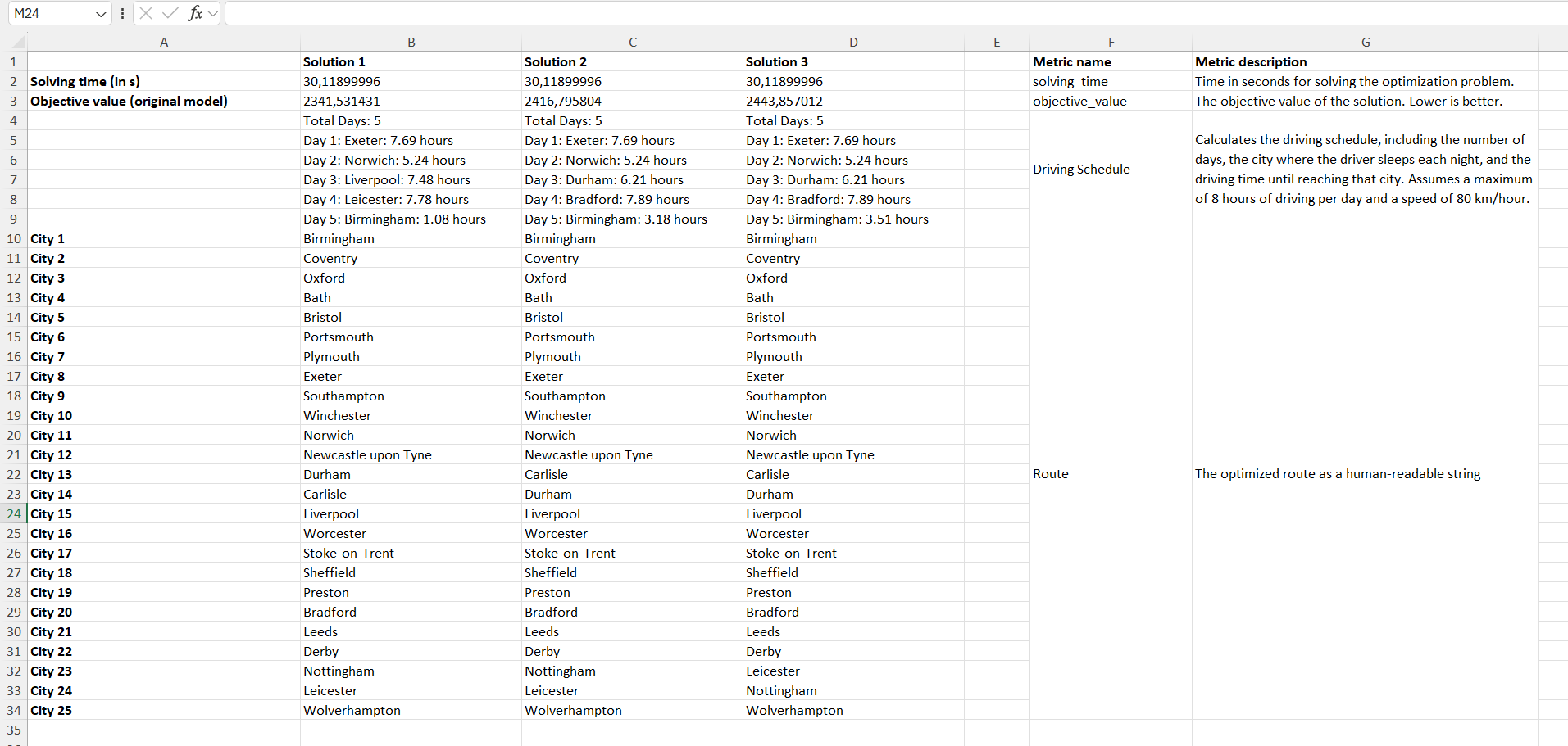
Adding a Metric
A metric is a quantitative measure that summarizes a key aspect of your optimization model’s performance. In our context, a metric function extracts and formats information from the model's inputs and outputs, presenting the results in an easily understandable format. Metrics help users quickly grasp the quality and characteristics of a solution without having to interpret raw numerical data.
A metric function must take as inputs the three parameters (p, c, x) and return two lists
of equal size: one containing labels (a list of strings) and the other containing corresponding values.
In our demo below, the metric reconstructs the optimized route as a human-readable string by mapping
the positions in the route back to city names.
def metric(p, c, x):
    all_city_names = [
        "Birmingham", "Leeds", "Sheffield", "Manchester", "Liverpool", "Bristol",
        "Newcastle upon Tyne", "Leicester", "Coventry", "Bradford",
        "Kingston upon Hull", "Stoke-on-Trent", "Wolverhampton", "Nottingham",
        "Derby", "Southampton", "Portsmouth", "Plymouth", "Exeter", "Norwich",
        "Chester", "Durham", "Winchester", "Gloucester", "Worcester", "Bath",
        "Preston", "Oxford", "Cambridge", "Carlisle"
    ]
    sel = [i for i, flag in enumerate(p["cities"]) if flag == 1]
    n = len(sel)
    order = [None] * n
    for ci in range(n):
        for pos in range(n):
            if x["x"][ci,pos] > 0.5:
                order[pos] = ci
                break
    labels = [f"City {i+1}" for i in range(n)]
    values = [all_city_names[ sel[ci] ] for ci in order]
    return labels, values

model.add_metric("Route", metric, explanation="The optimized route as a human-readable string")

model.generate_AI_metric(
    user_request=(
        "Please generate a metric that prints how many days it takes for the route if you drive max 8h per day "
        "and always sleep in one of the cities. Further tell me for each night in which city I will sleep "
        "and after how many hours of driving during the day I arrive there. Note that I can drive 80km per hour."
    )
)
model.print_all_metric_names()
model.upload()
When you run this model in the GUI and click on "Summary," an Excel spreadsheet will open displaying the metrics for each solution.
Adding Scripts
You can enhance your model by adding four types of custom scripts. These scripts enable you to integrate external data, visualize results, export solutions, and compute real-world objective values.
read(): A custom Python function that retrieves a problem instance (p).view(p, c, x): A function for representing or visualizing the solution in a user-friendly manner.write(p, c, x): A function that writes the solution back into other parts of your IT systems.objective(p, c, x): A function that computes and retrieves a real-world objective value for a given solutionx.
Below is a demonstration of how to integrate custom scripts into our TSP Pyomo model:
def read():
    arr = np.array([1]*20 + [0]*10)
    np.random.shuffle(arr)
    return {"cities": arr}

def view(p, c, x):
    all_city_names = [
        "Birmingham", "Leeds", "Sheffield", "Manchester", "Liverpool", "Bristol",
        "Newcastle upon Tyne", "Leicester", "Coventry", "Bradford",
        "Kingston upon Hull", "Stoke-on-Trent", "Wolverhampton", "Nottingham",
        "Derby", "Southampton", "Portsmouth", "Plymouth", "Exeter", "Norwich",
        "Chester", "Durham", "Winchester", "Gloucester", "Worcester", "Bath",
        "Preston", "Oxford", "Cambridge", "Carlisle"
    ]
    city_coords = {
        "Birmingham": (52.48142, -1.89983), "Leeds": (53.79648, -1.54785),
        "Sheffield": (53.38297, -1.46590), "Manchester": (53.48095, -2.23743),
        "Liverpool": (53.41058, -2.97794), "Bristol": (51.45523, -2.59665),
        "Newcastle upon Tyne": (54.97328, -1.61396), "Leicester": (52.63860, -1.13169),
        "Coventry": (52.40656, -1.51217), "Bradford": (53.79391, -1.75206),
        "Kingston upon Hull": (53.74460, -0.33525), "Stoke-on-Trent": (53.00415, -2.18538),
        "Wolverhampton": (52.58547, -2.12296), "Nottingham": (52.95360, -1.15047),
        "Derby": (52.92277, -1.47663), "Southampton": (50.90395, -1.40428),
        "Portsmouth": (50.79899, -1.09125), "Plymouth": (50.37153, -4.14305),
        "Exeter": (50.72360, -3.52751), "Norwich": (52.62783, 1.29834),
        "Chester": (53.19050, -2.89189), "Durham": (54.77676, -1.57566),
        "Winchester": (51.06513, -1.31870), "Gloucester": (51.86568, -2.24310),
        "Worcester": (52.18935, -2.22001), "Bath": (51.37510, -2.36172),
        "Preston": (53.76282, -2.70452), "Oxford": (51.75222, -1.25596),
        "Cambridge": (52.20000, 0.11667), "Carlisle": (54.89510, -2.93820)
    }
    sel = [i for i, flag in enumerate(p["cities"]) if flag == 1]
    n = len(sel)
    order = [None]*n
    for ci in range(n):
        for pos in range(n):
            if x["x"][ci,pos] > 0.5:
                order[pos] = ci
                break
    route = [all_city_names[ sel[ci] ] for ci in order] + [all_city_names[ sel[order[0]] ]]
    points = [city_coords[c] for c in route if c in city_coords]
    m = folium.Map(location=points[0], zoom_start=6)
    for city, pt in zip(route, points):
        folium.Marker(pt, popup=city).add_to(m)
    folium.PolyLine(locations=points, weight=2.5, opacity=1).add_to(m)
    html = Path.home()/"Documents"/"map.html"
    m.save(html)
    webbrowser.open("file://" + str(html))

def write(p, c, x):
    print("Processing and storing the chosen solution x with your own code.")

def objective(p, c, x):
    print("Retrieving the actual objective value from external IT sources.")
    return 42

model.add_read_script(read)
model.add_view_script(view)
model.add_write_script(write)
model.add_objective_script(objective)
model.upload()
Video Tutorial
This is the complete code from all four previous sections—including a README, a custom metric, an AI-generated metric, and scripts for read, view, write, and objective.
The video tutorial below uses the model created with this code.
from causara import *
import causara
import numpy as np
from pyomo.environ import ConcreteModel, Var, RangeSet, Constraint, Objective, Binary, minimize
import folium
import webbrowser
from pathlib import Path


def pyomo_model(p, c):
    selected = [i for i, flag in enumerate(p["cities"]) if flag == 1]
    n = len(selected)
    m = ConcreteModel()
    m.I = RangeSet(0, n-1)
    m.J = RangeSet(0, n-1)
    m.x = Var(m.I, m.J, domain=Binary)
    m.city_to_pos = Constraint(m.I, rule=lambda m,i: sum(m.x[i,j] for j in m.J) == 1)
    m.pos_to_city = Constraint(m.J, rule=lambda m,j: sum(m.x[i,j] for i in m.I) == 1)
    m.start_fixed = Constraint(expr=m.x[0,0] == 1)
    expr = 0
    for i1 in m.I:
        c1 = selected[i1]
        for j1 in m.J:
            for i2 in m.I:
                c2 = selected[i2]
                for j2 in m.J:
                    if j2 == j1 + 1 or (j1 == 0 and j2 == n-1):
                        expr += c["distance"][c1][c2] * m.x[i1,j1] * m.x[i2,j2]
    m.objective = Objective(expr=expr, sense=minimize)
    return m


def get_decision_vars(p, c):
    sel = [i for i, flag in enumerate(p["cities"]) if flag == 1]
    dv = DecisionVars()
    dv.add_binary_vars("x", (len(sel), len(sel)))
    return dv


model = Model(key="your_key", model_name="TSP_Tutorial")
model.compile(get_decision_vars, pyomo_func=pyomo_model, c=causara.Demos.TSP_real_data.c)
model.set_time_limit(time_limit=30)

cities = [
    "Birmingham", "Leeds", "Sheffield", "Manchester", "Liverpool", "Bristol",
    "Newcastle upon Tyne", "Leicester", "Coventry", "Bradford",
    "Kingston upon Hull", "Stoke-on-Trent", "Wolverhampton", "Nottingham",
    "Derby", "Southampton", "Portsmouth", "Plymouth", "Exeter", "Norwich",
    "Chester", "Durham", "Winchester", "Gloucester", "Worcester", "Bath",
    "Preston", "Oxford", "Cambridge", "Carlisle"
]
model.set_README(
    f"This is a classic TSP problem. p['cities'] is a binary vector of length 30 where "
    f"p['cities'][i] = 1 indicates that city i should be part of the route. "
    f"The cities are: {cities}. The route must be closed, so always consider the time going "
    f"from the last city back to the first city."
)

def metric(p, c, x):
    all_city_names = [
        "Birmingham", "Leeds", "Sheffield", "Manchester", "Liverpool", "Bristol",
        "Newcastle upon Tyne", "Leicester", "Coventry", "Bradford",
        "Kingston upon Hull", "Stoke-on-Trent", "Wolverhampton", "Nottingham",
        "Derby", "Southampton", "Portsmouth", "Plymouth", "Exeter", "Norwich",
        "Chester", "Durham", "Winchester", "Gloucester", "Worcester", "Bath",
        "Preston", "Oxford", "Cambridge", "Carlisle"
    ]
    sel = [i for i, flag in enumerate(p["cities"]) if flag == 1]
    n = len(sel)
    order = [None]*n
    for ci in range(n):
        for pos in range(n):
            if x["x"][ci,pos] > 0.5:
                order[pos] = ci
                break
    labels = [f"City {i+1}" for i in range(n)]
    values = [all_city_names[ sel[ci] ] for ci in order]
    return labels, values

model.add_metric("Route", metric, explanation="The optimized route as a human-readable string")

model.generate_AI_metric(
    user_request=(
        "Please generate a metric that prints how many days it takes for the route if you drive max 8h per day "
        "and always sleep in one of the cities. Further tell me for each night in which city I will sleep "
        "and after how many hours of driving during the day I arrive there. Note that I can drive 80km per hour."
    )
)
model.print_all_metric_names()

def read():
    arr = np.array([1]*20 + [0]*10)
    np.random.shuffle(arr)
    return {"cities": arr}

def view(p, c, x):
    all_city_names = [
        "Birmingham", "Leeds", "Sheffield", "Manchester", "Liverpool", "Bristol",
        "Newcastle upon Tyne", "Leicester", "Coventry", "Bradford",
        "Kingston upon Hull", "Stoke-on-Trent", "Wolverhampton", "Nottingham",
        "Derby", "Southampton", "Portsmouth", "Plymouth", "Exeter", "Norwich",
        "Chester", "Durham", "Winchester", "Gloucester", "Worcester", "Bath",
        "Preston", "Oxford", "Cambridge", "Carlisle"
    ]
    city_coords = {
        "Birmingham": (52.48142, -1.89983), "Leeds": (53.79648, -1.54785),
        "Sheffield": (53.38297, -1.46590), "Manchester": (53.48095, -2.23743),
        "Liverpool": (53.41058, -2.97794), "Bristol": (51.45523, -2.59665),
        "Newcastle upon Tyne": (54.97328, -1.61396), "Leicester": (52.63860, -1.13169),
        "Coventry": (52.40656, -1.51217), "Bradford": (53.79391, -1.75206),
        "Kingston upon Hull": (53.74460, -0.33525), "Stoke-on-Trent": (53.00415, -2.18538),
        "Wolverhampton": (52.58547, -2.12296), "Nottingham": (52.95360, -1.15047),
        "Derby": (52.92277, -1.47663), "Southampton": (50.90395, -1.40428),
        "Portsmouth": (50.79899, -1.09125), "Plymouth": (50.37153, -4.14305),
        "Exeter": (50.72360, -3.52751), "Norwich": (52.62783, 1.29834),
        "Chester": (53.19050, -2.89189), "Durham": (54.77676, -1.57566),
        "Winchester": (51.06513, -1.31870), "Gloucester": (51.86568, -2.24310),
        "Worcester": (52.18935, -2.22001), "Bath": (51.37510, -2.36172),
        "Preston": (53.76282, -2.70452), "Oxford": (51.75222, -1.25596),
        "Cambridge": (52.20000, 0.11667), "Carlisle": (54.89510, -2.93820)
    }
    sel = [i for i, flag in enumerate(p["cities"]) if flag == 1]
    n = len(sel)
    order = [None]*n
    for ci in range(n):
        for pos in range(n):
            if x["x"][ci,pos] > 0.5:
                order[pos] = ci
                break
    route = [all_city_names[ sel[ci] ] for ci in order] + [all_city_names[ sel[order[0]] ]]
    points = [city_coords[c] for c in route if c in city_coords]
    m = folium.Map(location=points[0], zoom_start=6)
    for city, pt in zip(route, points):
        folium.Marker(pt, popup=city).add_to(m)
    folium.PolyLine(locations=points, weight=2.5, opacity=1).add_to(m)
    html = Path.home()/"Documents"/"map.html"
    m.save(html)
    webbrowser.open("file://" + str(html))

def write(p, c, x):
    print("Processing and storing the chosen solution x with your own code.")

def objective(p, c, x):
    print("Retrieving the actual objective value from external IT sources.")
    return 42

model.add_read_script(read)
model.add_view_script(view)
model.add_write_script(write)
model.add_objective_script(objective)
model.upload()
You can start the causara GUI using the following command:
python -c "import causara; causara.GUI()"
You can also create a shortcut on the Desktop using the command:
python -c "import causara; causara.create_shortcut()"